Chapter 33 — Mixture of Experts (MoE)
“Why activate all 600 billion parameters for every token when only 100 billion are needed? MoE models are sparse — they think with a fraction of their brain.”
Dense vs Sparse Models
- Every parameter used for every token
- 70B params → 70B active per token
- Training FLOP per token: 6 × 70B = 420 GFLOP
- Memory: all 70B params loaded
- Only 2 of 8 FFN experts active per token
- 46.7B total params → ~12.9B active per token
- Training FLOP per token: 6 × 12.9B = 77 GFLOP
- Memory: all 46.7B params must be loaded
The key insight: MoE gives you the quality of a large model with the inference speed of a small model (if memory allows).
MoE Architecture
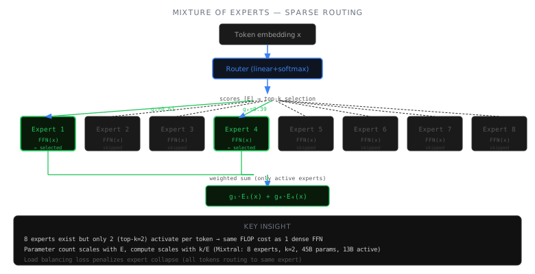
In a standard transformer, each layer has one FFN. In MoE, the FFN is replaced by N experts + a router:
Tensor Shapes
The Router
1
2
3
4
5
6
7
8
9
10
11
12
13
14
15
16
17
18
19
import torch
import torch.nn as nn
import torch.nn.functional as F

class TopKRouter(nn.Module):
    def __init__(self, d_model, n_experts, top_k=2):
        super().__init__()
        self.gate = nn.Linear(d_model, n_experts, bias=False)
        self.top_k = top_k

    def forward(self, x):
        # x: [B, T, d]
        logits = self.gate(x)                    # [B, T, n_experts]

        # Select top-K experts per token
        top_k_logits, top_k_indices = logits.topk(self.top_k, dim=-1)
        top_k_weights = F.softmax(top_k_logits, dim=-1)  # [B, T, K]

        return top_k_weights, top_k_indices
Load Balancing
Without intervention, the router collapses — sending most tokens to a few “popular” experts while others are idle. This is solved with an auxiliary load balancing loss:
\[L_{\text{balance}} = \alpha \cdot n_{\text{experts}} \cdot \sum_{i=1}^{n_{\text{experts}}} f_i \cdot P_i\]Where:
- $f_i$ = fraction of tokens routed to expert $i$
- $P_i$ = average router probability for expert $i$
- $\alpha$ = balance loss weight (typically 0.01)
This loss encourages uniform distribution of tokens across experts.
Simple MoE Layer Implementation
1
2
3
4
5
6
7
8
9
10
11
12
13
14
15
16
17
18
19
20
21
22
23
24
25
26
27
28
29
30
class MoELayer(nn.Module):
    def __init__(self, d_model, d_ff, n_experts=8, top_k=2):
        super().__init__()
        self.router = TopKRouter(d_model, n_experts, top_k)
        self.experts = nn.ModuleList([
            SwiGLU_FFN(d_model, d_ff) for _ in range(n_experts)
        ])
        self.n_experts = n_experts
        self.top_k = top_k

    def forward(self, x):
        B, T, d = x.shape
        weights, indices = self.router(x)    # [B,T,K], [B,T,K]

        # Flatten for routing
        x_flat = x.view(-1, d)               # [B*T, d]
        output = torch.zeros_like(x_flat)     # [B*T, d]

        for k in range(self.top_k):
            expert_indices = indices[:, :, k].reshape(-1)    # [B*T]
            expert_weights = weights[:, :, k].reshape(-1, 1) # [B*T, 1]

            for e in range(self.n_experts):
                mask = (expert_indices == e)
                if mask.any():
                    expert_input = x_flat[mask]
                    expert_output = self.experts[e](expert_input)
                    output[mask] += expert_weights[mask] * expert_output

        return output.view(B, T, d)
In production, this loop is replaced by optimized scatter/gather operations (e.g., Megablocks library).
Notable MoE Models
| Model | Total Params | Active Params | Experts | Top-K | Architecture Notes |
|---|---|---|---|---|---|
| Mixtral 8×7B | 46.7B | 12.9B | 8 | 2 | Every FFN is MoE. Sliding window attention. |
| Mixtral 8×22B | 141B | 39B | 8 | 2 | Larger experts. |
| DeepSeek-V2 | 236B | 21B | 160 | 6 | Fine-grained experts + shared expert. MLA attention. |
| DeepSeek-V3 | 671B | 37B | 256 | 8 | 256 routed + 1 shared expert per layer |
| Qwen2.5-MoE | 14.3B | 2.7B | 60 | 4 | Fine-grained, shared + routed experts |
| DBRX | 132B | 36B | 16 | 4 | Databricks, fine-grained experts |
| Switch Transformer | 1.6T | ~1.6B | 2048 | 1 | Google, top-1 routing for efficiency |
| Grok-1 | 314B | ~86B | 8 | 2 | xAI |
Fine-Grained Experts (DeepSeek Approach)
DeepSeek splits each expert into smaller “fine-grained” experts and adds a shared expert that always activates:
This design gives better expert utilization and reduces the load balancing problem.
MoE KV-Cache
An important practical point: MoE does not affect the KV-cache. Attention layers are shared (not sparse) — only the FFN is replaced by experts. This means:
- KV-cache size is identical to a dense model with the same attention dimensions
- Memory calculations from Chapter 17 apply directly
- The total model memory = attention params + all expert params (even though only K are active)
This creates a unique memory profile: MoE models need lots of memory for weights but have the same KV-cache footprint as their “active parameter” equivalent.
MoE Challenges
| Challenge | Impact | Mitigation |
|---|---|---|
| Memory: all experts must be loaded | 46.7B params for Mixtral (vs 12.9B active) | Quantization, expert offloading |
| Load imbalance: popular experts get overwhelmed | Training instability, wasted compute | Auxiliary loss, expert capacity limits |
| All-to-All communication: tokens must be routed across GPUs | Training bottleneck in distributed settings | Expert parallelism, careful placement |
| Fine-tuning: which experts to update? | LoRA on all experts is expensive | Shared expert + selective expert LoRA |
What’s Next
MoE shows that not all model architectures need to be dense transformers. The next chapter explores more radical departures — State Space Models (SSMs) and other alternatives to attention-based architectures.
← Previous: Chapter 32 — Scaling Laws & Emergent Abilities · Next: Chapter 34 — SSMs & Beyond Transformers →
Last updated: April 2026