Chapter 20 — Quantization Fundamentals
“Quantization is the art of throwing away precision strategically — keeping what matters and discarding what doesn’t.”
What Is Quantization?
Quantization maps high-precision floating-point values to lower-precision integers. For LLMs, this typically means FP16 → INT8 or INT4, reducing memory and enabling faster inference.
\[x_q = \text{round}\!\left(\frac{x}{s}\right) + z\]where $s$ = scale factor, $z$ = zero point, and $x_q$ is the quantized integer value.
Dequantization (at inference time): $\hat{x} = s \cdot (x_q - z)$
Symmetric vs Asymmetric Quantization
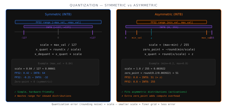
- Zero point z = 0 (no offset)
- Scale: s = max(|x|) / (2^(b-1) - 1)
- Range: [-127, 127] for INT8
- Simpler, faster dequantization
- Wastes range if distribution is skewed
- Zero point z ≠ 0 (shifted)
- Scale: s = (max(x) - min(x)) / (2^b - 1)
- Zero point: z = round(-min(x) / s)
- Full range utilization
- Better for skewed distributions
1
2
3
4
5
6
7
8
9
10
11
12
13
14
15
16
17
18
19
20
import torch

def symmetric_quantize(x, bits=8):
    """Symmetric quantization — zero-centered."""
    qmax = 2 ** (bits - 1) - 1                    # 127 for INT8
    scale = x.abs().max() / qmax
    x_q = torch.round(x / scale).clamp(-qmax, qmax).to(torch.int8)
    return x_q, scale

def symmetric_dequantize(x_q, scale):
    """Dequantize back to float."""
    return x_q.float() * scale

# Example
w = torch.randn(4096, 4096)                       # FP32 weight matrix
w_q, scale = symmetric_quantize(w, bits=8)
w_hat = symmetric_dequantize(w_q, scale)           # Reconstructed
print(f"Original: {w.nbytes / 1e6:.1f} MB")       # 67.1 MB
print(f"Quantized: {w_q.nbytes / 1e6:.1f} MB")    # 16.8 MB (4× smaller)
print(f"Max error: {(w - w_hat).abs().max():.6f}") # Small reconstruction error
Quantization Granularity
Where you compute scales dramatically affects quality:
Effective bits per value with group size 128: INT4 + scales + zeros ≈ 4.25 bits (the overhead from storing scales is small).
PTQ vs QAT
- Quantize after training is complete
- Uses calibration dataset (~128–512 samples)
- No additional training needed
- Fast: minutes to hours
- Lower quality at extreme compression (INT3/2)
- Simulate quantization during training
- Model adapts to quantization noise
- Requires training infrastructure
- Slow: full training cost
- Best quality at any bit-width
For LLMs, PTQ dominates because models are expensive to retrain. QAT methods like BitNet train from scratch.
Calibration Strategies
PTQ methods need a calibration dataset to determine quantization parameters (scales, zero points). The choice of calibration strategy matters:
| Strategy | Description | Quality |
|---|---|---|
| Min-Max | Use observed min/max of activations | Baseline |
| Percentile | Clip to 99.9th percentile (ignore outliers) | Better |
| MSE | Minimize reconstruction error (MSE) per layer | Best |
| Entropy | Minimize KL divergence between original and quantized | Good |
What Gets Quantized
When to use each:
- Weight-only: most LLM inference (decode is memory-bandwidth bound — smaller weights = faster reads)
- Weight + activation: latency-sensitive serving, batch inference (prefill is compute-bound)
- KV-cache: long-context serving, high-throughput scenarios
The Outlier Problem
LLM activations have massive outliers — a few channels with values 100× larger than average. These outliers make naive quantization fail because the scale is dominated by outliers, leaving most values underrepresented.
1
2
3
4
5
6
7
# Typical activation distribution in a transformer
# 99% of values: [-3, 3]
# 0.1% outlier channels: [-100, 100]
# If we quantize to [-127, 127] with max=100:
#   scale = 100/127 ≈ 0.79
#   A value of 1.0 maps to round(1.0/0.79) = 1 → dequant = 0.79
#   Quantization error of 0.21 — over 20% for typical values!
This is why methods like SmoothQuant, GPTQ, and AWQ were invented — they’re all different strategies for handling outliers. See Chapter 21.
What’s Next
With the fundamentals in place, the next chapter surveys the full landscape of quantization techniques — from GPTQ and AWQ to SmoothQuant and BitNet, with a master comparison table.
← Previous: Chapter 19 — Data Types & Numerical Precision · Next: Chapter 21 — Quantization Techniques →
Last updated: April 2026