Chapter 32 — Scaling Laws & Emergent Abilities
“The remarkable thing about scaling laws is how predictable they are. The remarkable thing about emergent abilities is how unpredictable they are.”
Neural Scaling Laws
The performance of language models follows predictable power-law relationships with compute, data, and parameters.
The Kaplan Scaling Laws (2020)
OpenAI’s initial scaling laws found that loss decreases as a power law in each of three factors (holding the others fixed):
\[L(N) \propto N^{-\alpha_N}, \quad L(D) \propto D^{-\alpha_D}, \quad L(C) \propto C^{-\alpha_C}\]Where:
- N = number of parameters
- D = number of training tokens
- C = compute budget (FLOPs)
- L = cross-entropy loss
Key finding: parameters matter more than data. For a fixed compute budget, it’s better to train a larger model on less data.
Chinchilla Scaling Laws (2022)
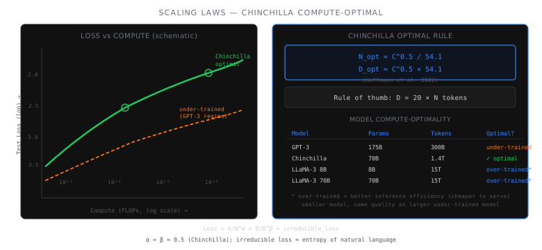
DeepMind’s Hoffmann et al. challenged the Kaplan findings. They showed that data and parameters should scale equally:
- Scale parameters faster than data
- GPT-3 175B trained on 300B tokens
- Ratio: ~1.7 tokens per parameter
- "Bigger model, less data"
- Scale parameters and data equally
- Chinchilla 70B trained on 1.4T tokens
- Ratio: ~20 tokens per parameter
- "For N params, train on ~20N tokens"
Chinchilla (70B, 1.4T tokens) outperformed Gopher (280B, 300B tokens) despite being 4× smaller, using the same compute. This reshaped how models are trained.
Practical Compute-Optimal Ratios
| Model Size | Chinchilla-Optimal Tokens | Compute (C ≈ 6ND) |
|---|---|---|
| 1B | 20B | 1.2 × 10²⁰ |
| 7B | 140B | 5.9 × 10²¹ |
| 13B | 260B | 2.0 × 10²² |
| 70B | 1.4T | 5.9 × 10²³ |
| 405B | 8.1T | 2.0 × 10²⁵ |
Beyond Chinchilla
In practice, modern models are trained well beyond Chinchilla-optimal:
| Model | Parameters | Training Tokens | Tokens/Param | Chinchilla-Optimal? |
|---|---|---|---|---|
| Chinchilla | 70B | 1.4T | 20× | ✅ Yes (by design) |
| LLaMA-1 65B | 65B | 1.4T | 21× | ≈ Yes |
| LLaMA-2 70B | 70B | 2T | 29× | Over-trained |
| LLaMA-3 8B | 8B | 15T | 1,875× | Way over-trained |
| LLaMA-3 70B | 70B | 15T | 214× | Way over-trained |
| Mistral 7B | 7B | ~8T (est.) | ~1,100× | Way over-trained |
Why over-train? Chinchilla optimizes for training compute. But inference compute dominates total cost. A smaller model trained longer is cheaper to serve — LLaMA-3-8B (15T tokens) is far cheaper to deploy than a Chinchilla-optimal 70B model with similar quality.
Scaling Law for Inference
The inference-optimal perspective (Sardana & Frankle, 2023):
\[L = \left(\frac{N_0}{N}\right)^{\alpha_N} + \left(\frac{D_0}{D}\right)^{\alpha_D}\]When you account for total lifetime cost (training + inference), smaller models trained on more data are often preferable. This explains the trend toward “smaller but well-trained” models.
Emergent Abilities
Some capabilities appear to emerge suddenly at a certain scale rather than improving gradually:
Documented Emergent Abilities
| Ability | Approximate Emergence Scale |
|---|---|
| In-context learning (few-shot) | ~1B+ params |
| Chain-of-thought reasoning | ~10B+ (effective with prompting at ~60B+) |
| Multi-step arithmetic | ~50B+ |
| Code generation | ~10B+ (usable), ~70B+ (competitive) |
| Instruction following | ~7B+ (with alignment), ~70B+ (robust) |
| Theory of mind (simple) | ~100B+ (debated) |
The “Mirage” Debate
Schaeffer, Miranda, and Sanborn (2023) argued that emergence is a measurement artifact:
- Some tasks show clear phase transitions
- CoT prompting only works above a threshold
- Qualitative behavior changes at scale
- Not just a smooth improvement
- Using continuous metrics (log-prob) instead of exact match → smooth curves
- Apparent jumps are artifacts of discrete metrics
- Token-level accuracy improves smoothly; task-level accuracy appears to "jump"
- Matters of how you measure, not what the model can do
The resolution: both are partly right. Token-level capabilities improve smoothly, but some composite behaviors (multi-step reasoning, following complex instructions) genuinely require crossing a capability threshold.
Implications for Practice
- Training budget: If you know your compute budget C, you can estimate optimal N and D
- Over-training is good for deployment: Train smaller models on more data for cheaper inference
- Smaller models improve with better data: Data quality scaling (FineWeb, DCLM) can substitute for model size
- Don’t expect emergence from small models: Some capabilities genuinely require scale
- Predict before you train: Use scaling laws to extrapolate from small experiments
1
2
3
4
5
6
7
8
9
10
11
12
13
14
15
16
17
# Simple scaling law fit (toy example)
import numpy as np
from scipy.optimize import curve_fit

# Observed loss at different parameter counts
params = [125e6, 350e6, 1.3e9, 6.7e9, 13e9]
losses = [3.64, 3.13, 2.68, 2.28, 2.11]

def scaling_law(N, A, alpha):
    return A * N ** (-alpha)

popt, pcov = curve_fit(scaling_law, params, losses)
print(f"L(N) = {popt[0]:.2f} × N^(-{popt[1]:.4f})")

# Predict loss at 70B
predicted_loss = scaling_law(70e9, *popt)
print(f"Predicted loss at 70B: {predicted_loss:.2f}")
What’s Next
Scaling laws tell us how big to make a model. But what if we could make a model effectively bigger without proportionally increasing compute? The next chapter covers Mixture of Experts (MoE) — sparse models that activate only a fraction of their parameters.
← Previous: Chapter 31 — Serving & Deployment · Next: Chapter 33 — Mixture of Experts →
Last updated: April 2026