Chapter 3 — The Transformer
“Attention is all you need.” — Vaswani et al., 2017
The Architecture That Changed Everything
The transformer is the architecture behind every modern LLM. Introduced in 2017 for machine translation, its purely attention-based design replaced recurrence and convolution with a mechanism that can attend to all positions in parallel. This chapter walks through every component with tensor shapes at each step.
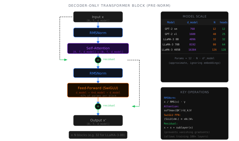
A transformer model is simply N of these blocks stacked sequentially. LLaMA-3-8B uses N = 32 blocks; LLaMA-3-70B uses N = 80.
Tensor Flow Through a Full Model
The hidden dimension stays constant at d_model through all transformer blocks. Only the final linear projection (the “LM head”) changes the dimension to the vocabulary size.
Component Deep Dive
Residual Connections
Every sub-layer (attention and FFN) uses a residual (skip) connection: the input to the sub-layer is added to its output. This enables gradient flow through deep networks and lets each layer learn a delta rather than a full transformation:
\[\text{output} = x + \text{SubLayer}(\text{Norm}(x))\]Without residual connections, training a 32-layer or 80-layer model would be extremely difficult due to vanishing gradients.
Layer Normalization vs RMS Normalization
Normalization stabilizes training by keeping activations in a consistent range.
LayerNorm (original transformer, BERT): \(\text{LayerNorm}(x) = \frac{x - \mu}{\sqrt{\sigma^2 + \epsilon}} \cdot \gamma + \beta\)
RMSNorm (LLaMA, Mistral, modern models): \(\text{RMSNorm}(x) = \frac{x}{\sqrt{\frac{1}{d}\sum_{i=1}^{d} x_i^2 + \epsilon}} \cdot \gamma\)
RMSNorm drops the mean-centering and bias, making it ~10–15% faster than LayerNorm with negligible quality difference. It’s the standard in modern LLMs.
| Property | LayerNorm | RMSNorm |
|---|---|---|
| Mean centering | Yes (−μ) | No |
| Learnable bias | Yes (β) | No |
| Learnable scale | Yes (γ) | Yes (γ) |
| Speed | Baseline | ~10–15% faster |
| Used by | BERT, GPT-2 | LLaMA, Mistral, Gemma |
Pre-Norm vs Post-Norm
The placement of normalization matters:
- x → Norm → SubLayer → + residual
- More stable training
- Used by LLaMA, GPT-3, Mistral
- Gradients flow directly through residuals
- x → SubLayer → + residual → Norm
- Requires careful LR warmup
- Used by original Transformer, BERT
- Can produce slightly better results with care
1
2
3
4
5
6
7
8
9
10
11
12
import torch
import torch.nn as nn

class RMSNorm(nn.Module):
    def __init__(self, d_model, eps=1e-6):
        super().__init__()
        self.weight = nn.Parameter(torch.ones(d_model))
        self.eps = eps

    def forward(self, x):
        rms = torch.sqrt(torch.mean(x ** 2, dim=-1, keepdim=True) + self.eps)
        return x / rms * self.weight
Feed-Forward Network (FFN)
Each transformer block has a position-wise feed-forward network that operates independently on each token’s representation. It projects up to a larger dimension, applies a non-linearity, and projects back down:
Activation Functions
The FFN’s non-linearity determines what the model can learn:
| Activation | Formula | Used By |
|---|---|---|
| ReLU | $\max(0, x)$ | Original Transformer |
| GELU | $x \cdot \Phi(x)$ | GPT-2, BERT |
| SiLU (Swish) | $x \cdot \sigma(x)$ | LLaMA, Mistral |
| SwiGLU | $\text{SiLU}(xW_1) \otimes xW_3$ | LLaMA 2/3, Gemma |
SwiGLU (Shazeer, 2020) is the dominant choice in modern models. It uses a gated linear unit — one linear projection creates the “gate” while another creates the “value,” and they’re multiplied element-wise:
1
2
3
4
5
6
7
8
9
10
11
class SwiGLU_FFN(nn.Module):
    def __init__(self, d_model, d_ff):
        super().__init__()
        self.w_gate = nn.Linear(d_model, d_ff, bias=False)  # gate projection
        self.w_up   = nn.Linear(d_model, d_ff, bias=False)  # up projection
        self.w_down = nn.Linear(d_ff, d_model, bias=False)   # down projection

    def forward(self, x):  # x: [B, T, d_model]
        gate = torch.nn.functional.silu(self.w_gate(x))  # [B, T, d_ff]
        up = self.w_up(x)                                 # [B, T, d_ff]
        return self.w_down(gate * up)                      # [B, T, d_model]
Note that SwiGLU has 3 weight matrices instead of 2, so d_ff is typically set to 2/3 of what it would be with a standard FFN to keep the parameter count similar (e.g., 14336 instead of ~21845 for d_model=4096).
A Minimal Transformer Block
Combining all components (attention is a placeholder here — see Chapter 4):
1
2
3
4
5
6
7
8
9
10
11
12
13
14
15
16
17
18
19
20
21
22
23
24
25
26
27
28
29
30
31
32
class TransformerBlock(nn.Module):
    def __init__(self, d_model, n_heads, d_ff):
        super().__init__()
        self.attn_norm = RMSNorm(d_model)
        self.attn = MultiHeadAttention(d_model, n_heads)  # Chapter 4
        self.ffn_norm = RMSNorm(d_model)
        self.ffn = SwiGLU_FFN(d_model, d_ff)

    def forward(self, x, mask=None):
        # Pre-norm + attention + residual
        h = x + self.attn(self.attn_norm(x), mask=mask)   # [B, T, d_model]
        # Pre-norm + FFN + residual
        out = h + self.ffn(self.ffn_norm(h))               # [B, T, d_model]
        return out

class Transformer(nn.Module):
    def __init__(self, vocab_size, d_model, n_layers, n_heads, d_ff):
        super().__init__()
        self.embed = nn.Embedding(vocab_size, d_model)
        self.layers = nn.ModuleList([
            TransformerBlock(d_model, n_heads, d_ff) for _ in range(n_layers)
        ])
        self.norm = RMSNorm(d_model)
        self.lm_head = nn.Linear(d_model, vocab_size, bias=False)

    def forward(self, input_ids, mask=None):
        x = self.embed(input_ids)           # [B, T, d_model]
        for layer in self.layers:
            x = layer(x, mask=mask)          # [B, T, d_model]
        x = self.norm(x)                     # [B, T, d_model]
        logits = self.lm_head(x)             # [B, T, vocab_size]
        return logits
Parameter Count
Understanding where parameters live in a transformer:
| Component | Shape | Count (LLaMA-3-8B) |
|---|---|---|
| Embedding | [128256, 4096] | 525M |
| Per block: Q, K, V projections | [4096, 4096] × 3 | 50M |
| Per block: Output projection | [4096, 4096] | 17M |
| Per block: FFN (gate, up, down) | [4096, 14336] × 3 | 176M |
| Per block: 2× RMSNorm | [4096] × 2 | 8K |
| Final RMSNorm | [4096] | 4K |
| Total (32 blocks) | ~8B |
The FFN layers dominate — they account for roughly 2/3 of all parameters in each block. Attention parameters are about 1/3. The embedding matrix is large but shared with the LM head (weight tying).
What’s Next
The transformer block contains two sub-layers, and we’ve covered the FFN in detail. The next chapter dives deep into the other — and arguably more important — component: attention.
← Previous: Chapter 2 — Embeddings · Next: Chapter 4 — SDPA & Multi-Head Attention →
Last updated: April 2026