Chapter 2 — Embeddings & Representations
“You shall know a word by the company it keeps.” — J.R. Firth, 1957
From IDs to Vectors
After tokenization (see Appendix B), each token is an integer ID — say, 4037 for the token “token”. But a model can’t learn meaningful patterns from raw integers. The embedding layer maps each token ID to a dense vector in a continuous space where similar tokens live near each other.
The embedding matrix E has shape [V, d_model] — one row per token in the vocabulary. Looking up a token is simply indexing into this matrix:
For LLaMA-3-8B: V = 128,256 and d_model = 4,096, so the embedding matrix alone is 128,256 × 4,096 × 2 bytes (BF16) ≈ 1 GB.
1
2
3
4
5
6
7
8
9
10
11
12
13
14
import torch
import torch.nn as nn

vocab_size = 128256
d_model = 4096

# The embedding layer — a learnable lookup table
embedding = nn.Embedding(vocab_size, d_model)

# Input: batch of token IDs
token_ids = torch.tensor([[14658, 4211, 7963, 279]])  # [1, 4]
vectors = embedding(token_ids)                          # [1, 4, 4096]
print(f"Input shape:  {token_ids.shape}")   # [1, 4]
print(f"Output shape: {vectors.shape}")     # [1, 4, 4096]
The Evolution of Word Representations
One-Hot Encoding
The simplest representation: each word is a binary vector of length V with a single 1 at the word’s index. For a vocabulary of 128K tokens, each vector is 128K-dimensional and sparse. The dot product between any two different one-hot vectors is zero — the representation carries no semantic information.
Word2Vec and GloVe (Static Embeddings)
Word2Vec (Mikolov et al., 2013) demonstrated that training a simple neural network on “predict a word from its neighbors” produces vectors where semantic relationships are encoded as linear directions:
These embeddings are static — each word maps to one fixed vector regardless of context. “Bank” has the same embedding whether you’re talking about a river bank or a financial bank.
Contextual Embeddings (Transformers)
In modern LLMs, embeddings are contextual: the initial embedding lookup produces static vectors, but the transformer layers refine them based on the surrounding context. After multiple transformer layers, the representation for “bank” in “river bank” is completely different from “bank” in “bank account”. The initial embedding is just the starting point.
Positional Encodings
Attention (covered in Chapter 4) is inherently position-agnostic — it treats the input as a set, not a sequence. Without positional information, the model can’t distinguish “the cat sat on the mat” from “the mat sat on the cat”. Positional encodings inject sequence order.
Sinusoidal (Original Transformer)
The original “Attention Is All You Need” paper used fixed, non-learned sinusoidal functions:
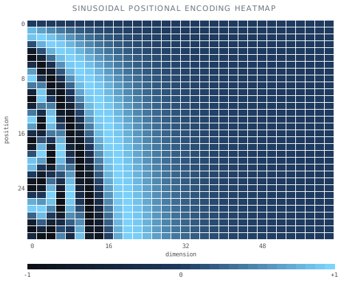
\[PE_{(pos, 2i)} = \sin\!\left(\frac{pos}{10000^{2i/d_{model}}}\right), \quad PE_{(pos, 2i+1)} = \cos\!\left(\frac{pos}{10000^{2i/d_{model}}}\right)\]Each position gets a unique d_model-dimensional pattern. The beauty: relative positions are captured as linear transformations, and the model can extrapolate to unseen lengths (in theory).
The heatmap below shows positions (rows) vs dimensions (columns). High-frequency oscillations in the early dimensions uniquely identify close positions; low-frequency oscillations in later dimensions encode long-range order.
1
2
3
4
5
6
7
8
9
10
11
12
13
import torch
import math

def sinusoidal_pe(max_len, d_model):
    pe = torch.zeros(max_len, d_model)
    position = torch.arange(0, max_len).unsqueeze(1).float()
    div_term = torch.exp(torch.arange(0, d_model, 2).float() * -(math.log(10000.0) / d_model))
    pe[:, 0::2] = torch.sin(position * div_term)
    pe[:, 1::2] = torch.cos(position * div_term)
    return pe  # [max_len, d_model]

pe = sinusoidal_pe(max_len=2048, d_model=512)  # [2048, 512]
print(f"Positional encoding shape: {pe.shape}")
Learned Positional Embeddings (GPT-2)
GPT-2 used a learned embedding table for positions — just like the token embedding but indexed by position (0, 1, 2, …, max_len-1). Simple and effective, but fixed to a maximum sequence length at training time.
1
2
3
4
5
6
7
8
9
# Learned positional embedding
max_seq_len = 2048
position_embedding = nn.Embedding(max_seq_len, d_model)  # [2048, 4096]

positions = torch.arange(0, seq_len).unsqueeze(0)  # [1, T]
pos_emb = position_embedding(positions)              # [1, T, d_model]

# Combine token + position embeddings
hidden = token_embedding(input_ids) + pos_emb  # [B, T, d_model]
RoPE — Rotary Position Embedding (LLaMA, Mistral, Qwen)
RoPE (Su et al., 2021) is the dominant positional encoding in modern LLMs. Instead of adding a position vector to the embedding, RoPE rotates the query and key vectors inside each attention head by an angle proportional to the token’s position. Because both Q and K are rotated the same way, the dot-product attention score naturally captures only the relative distance between positions — not absolute positions.
Core Idea: Rotation in 2D Subspaces
RoPE partitions each d_head-dimensional query/key vector into d_head/2 consecutive pairs of dimensions. For each pair (2i, 2i+1), it applies a 2D rotation matrix parameterised by the position index m and a base frequency $\theta_i$:
\[\begin{pmatrix} q_{2i}' \\ q_{2i+1}' \end{pmatrix} = \begin{pmatrix} \cos(m\theta_i) & -\sin(m\theta_i) \\ \sin(m\theta_i) & \cos(m\theta_i) \end{pmatrix} \begin{pmatrix} q_{2i} \\ q_{2i+1} \end{pmatrix}\]Where the base frequency for pair i is:
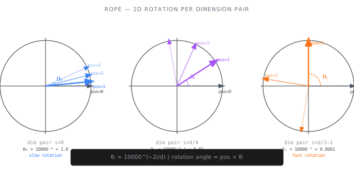
\[\theta_i = \frac{1}{10000^{2i/d_{head}}}\]This means each pair of dimensions rotates at a different angular speed — high-index pairs rotate slowly (long-range), low-index pairs rotate quickly (short-range).
Why Relative Position Falls Out Naturally
When two rotated vectors $q’$ (at position $m$) and $k’$ (at position $n$) are dot-producted in attention, the rotation angles cancel to leave only $(m - n)$:
\[q'^{\top} k' = \text{Re}\!\left[\sum_{i=0}^{d/2-1} q_{[i]} k_{[i]}^{*} e^{j(m-n)\theta_i}\right]\]The model never needs to learn absolute positions — relative offsets are built into the geometry.
Angle Rotation Visualization
The diagram below shows how the same query vector for position m=1 (vs m=0) rotates by different amounts across three frequency bands. Low-frequency pairs barely move; high-frequency pairs rotate nearly 90° per step.
Tensor Shapes
RoPE does not change the shape of Q or K — it only rotates the values in-place.
1
2
3
4
5
6
7
8
9
10
11
12
13
14
15
16
17
18
19
20
21
22
23
24
25
26
27
28
29
30
31
32
33
34
35
36
37
38
39
40
41
42
43
import torch

def rope_frequencies(d_head: int, max_len: int = 8192, base: float = 10000.0):
    """Precompute cosine and sine tables for RoPE.
    Returns cos, sin each of shape [max_len, d_head/2].
    """
    # θᵢ = 1 / base^(2i/d_head)  for i = 0, 1, ..., d_head/2 - 1
    i = torch.arange(0, d_head, 2).float()          # step 2 → d_head/2 elements
    theta = 1.0 / (base ** (i / d_head))             # [d_head/2]

    positions = torch.arange(max_len).float()         # [max_len]
    angles = torch.outer(positions, theta)            # [max_len, d_head/2]
    return torch.cos(angles), torch.sin(angles)       # each [max_len, d_head/2]


def apply_rope(x: torch.Tensor, cos: torch.Tensor, sin: torch.Tensor) -> torch.Tensor:
    """Apply RoPE to Q or K.
    x:   [B, H, T, d_head]
    cos: [T, d_head/2]
    sin: [T, d_head/2]
    Returns rotated tensor of same shape [B, H, T, d_head].
    """
    T, d_half = x.shape[2], x.shape[-1] // 2
    x1 = x[..., :d_half]                              # [B, H, T, d_head/2]
    x2 = x[..., d_half:]                              # [B, H, T, d_head/2]

    # Broadcast cos/sin from [T, d_half] → [1, 1, T, d_half]
    c = cos[:T].unsqueeze(0).unsqueeze(0)
    s = sin[:T].unsqueeze(0).unsqueeze(0)

    # Apply 2D rotation: [x1·cos − x2·sin, x2·cos + x1·sin]
    rotated = torch.cat([x1 * c - x2 * s, x2 * c + x1 * s], dim=-1)
    return rotated                                      # [B, H, T, d_head]


# Usage inside attention
d_head = 128
cos_cache, sin_cache = rope_frequencies(d_head, max_len=8192)

# q, k: [B, H, T, d_head]
q_rot = apply_rope(q, cos_cache, sin_cache)
k_rot = apply_rope(k, cos_cache, sin_cache)
# Then compute attention scores: q_rot @ k_rot.transpose(-1, -2) / sqrt(d_head)
RoPE Frequency Scaling (YaRN, LongRoPE, LLaMA-3 RoPE scaling)
The base frequency can be scaled to extend the context window beyond what the model was trained on. If a model was trained at 8K context with base=10000, multiplying the base (e.g., to base=500000) slows down all rotation frequencies, letting the model handle much longer sequences. LLaMA-3 uses base=500000 and LLaMA-3.1 extends context to 128K this way.
M-RoPE — Multimodal Rotary Position Embedding
M-RoPE (used in Qwen-VL2, LLaMA-3.2 Vision, and similar multimodal LLMs) extends RoPE to handle inputs that have multiple spatial or temporal dimensions — images, video frames, or interleaved text+image sequences.
The Problem with 1D RoPE for Images
A standard 1D RoPE assigns each token a single scalar position: token 0, 1, 2, 3… For text this is natural. But an image patch at row h, column w has two spatial coordinates. Flattening patches into a 1D sequence loses the 2D structure — the model can’t tell whether two adjacent patches are horizontally or vertically adjacent.
M-RoPE: Separate Frequency Bands per Axis
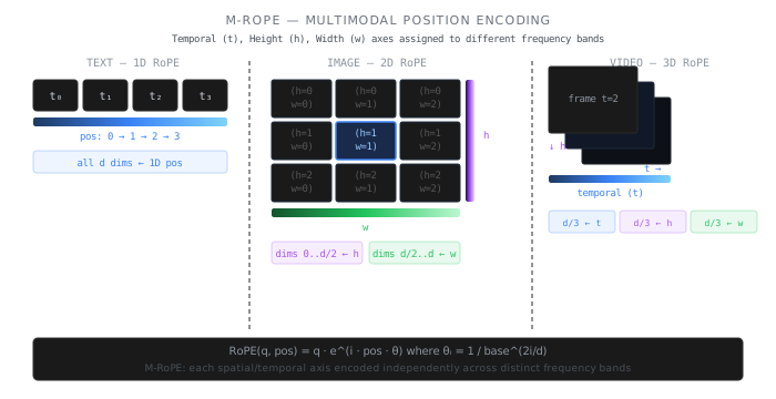
M-RoPE assigns different frequency bands (subsets of the d_head dimensions) to encode each axis independently:
| Modality | Axes | Dim allocation |
|---|---|---|
| Text | position | all d_head dims ← 1D pos |
| Image | height, width | d_head/2 dims ← h · θ, d_head/2 dims ← w · θ |
| Video | time, height, width | d_head/3 dims each ← t · θ, h · θ, w · θ |
Each token’s RoPE rotation is computed from its (t, h, w) coordinates rather than a single scalar index:
\[q' = R(t \cdot \theta_{\text{time}}) \cdot R(h \cdot \theta_{\text{height}}) \cdot R(w \cdot \theta_{\text{width}}) \cdot q\]For text tokens, the same position value is used for all three axes (t = h = w = seq_pos), so M-RoPE degrades gracefully to standard 1D RoPE.
M-RoPE Tensor Shapes
1
2
3
4
5
6
7
8
9
10
11
12
13
14
15
16
17
18
19
20
21
22
23
24
25
26
27
28
29
30
31
32
def mrope_image_frequencies(
    h_ids: torch.Tensor,    # [N] — row index of each patch
    w_ids: torch.Tensor,    # [N] — col index of each patch
    d_head: int,
    base: float = 10000.0
):
    """Compute M-RoPE angles for image patches.
    Returns cos, sin each of shape [N, d_head/2].
    Half the d_head dims encode height, half encode width.
    """
    d_half = d_head // 2
    d_quarter = d_half // 2                          # dims per spatial axis

    i = torch.arange(0, d_quarter * 2, 2).float()
    theta = 1.0 / (base ** (i / d_head))             # [d_quarter] base freqs

    h_angles = torch.outer(h_ids.float(), theta)     # [N, d_quarter]
    w_angles = torch.outer(w_ids.float(), theta)     # [N, d_quarter]

    # Interleave: first d_half dims ← height, second d_half dims ← width
    # [N, d_quarter] + [N, d_quarter] → [N, d_quarter*2] = [N, d_half]
    angles = torch.cat([h_angles, w_angles], dim=-1) # [N, d_half]
    return torch.cos(angles), torch.sin(angles)


# Example: 14×14 image (196 patches)
H, W = 14, 14
h_ids = torch.arange(H).repeat_interleave(W)        # [196]
w_ids = torch.arange(W).repeat(H)                   # [196]

cos_2d, sin_2d = mrope_image_frequencies(h_ids, w_ids, d_head=128)
# cos_2d, sin_2d: [196, 64] — applied to Q and K patches
ALiBi — Attention with Linear Biases
| ALiBi (Press et al., 2022) takes a different approach: no positional encoding at all. Instead, it adds a linear bias to attention scores based on the distance between query and key positions. Position i attending to position j gets a bias of $-m \cdot | i - j | $ where m is a head-specific slope. |
ALiBi has strong length extrapolation properties — models trained on short sequences can generalize to longer ones at inference without re-training.
Positional Encoding Comparison
| Method | Added Where | Relative Position | Length Extrapolation | Used By |
|---|---|---|---|---|
| Sinusoidal | Embedding output | Implicit (via rotation) | Moderate | Original Transformer |
| Learned | Embedding output | No | None (fixed max_len) | GPT-2, BERT |
| RoPE | Q, K in attention | Yes (rotation angle) | Good (with base scaling) | LLaMA, Mistral, Qwen, Gemma |
| M-RoPE | Q, K in attention | Yes (per axis) | Inherits from RoPE | Qwen-VL2, LLaMA-3.2 Vision |
| ALiBi | Attention scores | Yes (linear bias) | Strong | BLOOM, MPT |
Modern models overwhelmingly use RoPE (or M-RoPE for multimodal) due to its balance of performance, relative position awareness, and extensibility. The base frequency can be scaled for longer contexts — discussed further in Chapter 12.
Tying Embeddings
Many models tie the input embedding matrix with the output projection (the “LM head”). This means the matrix used to look up token embeddings is the same matrix used to project hidden states back to vocabulary logits:
\[\text{logits} = h \cdot E^T\]Where $h$ is the final hidden state [B, T, d_model] and $E^T$ is the transposed embedding matrix [d_model, V].
This halves the number of embedding parameters (significant when V is large) and enforces consistency — the output space matches the input space.
What’s Next
Embeddings give tokens their initial representations. The next chapter covers the architecture that transforms these representations into something powerful — the transformer.
Next: Chapter 3 — The Transformer →
Last updated: April 2026