Chapter 23 — Knowledge Distillation & QAD
“Distillation is the art of compressing a large model’s knowledge into a smaller one — and quantization-aware distillation pushes that compression further without sacrificing quality.”
Why Distillation?
Quantisation (Chapters 20–22) reduces memory by lowering numeric precision. Distillation takes a complementary approach: train a smaller student model to mimic a larger teacher model, transferring knowledge without requiring the student to go through expensive pre-training from scratch.
Knowledge Distillation — Fundamentals
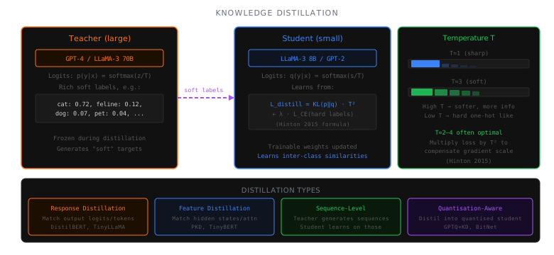
The Core Idea (Hinton et al., 2015)
A neural network trained on hard labels (one-hot targets) discards the probability mass it assigns to near-misses. A teacher model’s soft logits contain rich information about similarity structure:
Hard label (training signal from dataset):
1
target: [0, 0, 0, 1, 0, 0, ...]  ← "cat" is correct
Soft teacher label (richer signal):
1
2
teacher output: [0.001, 0.003, 0.002, 0.85, 0.09, 0.04, ...]
                          ↑ dog         ↑ cat   ↑ kitten
The soft distribution tells the student that “cat” is most likely, but “dog” and “kitten” are plausible — carrying far more information than a one-hot label.
Distillation Loss
The student is trained with a combination of:
-
Hard-target loss (standard cross-entropy against ground truth): \(\mathcal{L}_{\text{CE}} = -\sum_t \log p_S(x_t \mid x_{<t})\)
-
Soft KL divergence (student learns from teacher’s distribution): \(\mathcal{L}_{\text{KD}} = T^2 \cdot \text{KL}(p_T^{(T)} \| p_S^{(T)})\)
where temperature
Tsharpens/softens distributions andp^{(T)}means softmax at temperatureT. -
Combined objective: \(\mathcal{L} = (1 - \alpha)\mathcal{L}_{\text{CE}} + \alpha \mathcal{L}_{\text{KD}}\)
α ∈ [0,1]balances hard vs soft targets. Common:α = 0.5–0.9.
Temperature in Distillation
Temperature T controls the “softness” of the teacher distribution:
- T=1: standard softmax (sharp, peaked at top-1)
- T=4–10: softer distribution, more probability mass on near-misses — richer learning signal for the student
Tensor shapes during distillation:
| Tensor | Shape | Description |
|---|---|---|
| Teacher logits | [B, T, V] |
Raw logits before softmax |
| Soft teacher probs | [B, T, V] |
After softmax at temperature T |
| Student logits | [B, T, V] |
Student output |
| Soft student probs | [B, T, V] |
After softmax at temperature T |
| KL loss | scalar | Per-token divergence, averaged |
Types of Distillation for LLMs
Response-Based Distillation (Output Distillation)
The student learns from the teacher’s output token probabilities. This is the simplest form — only the final logits are used:
1
2
3
Teacher: generates logits z_T ∈ [B, T, V]
Student: generates logits z_S ∈ [B, T, V]
Loss: KL(softmax(z_T/τ) || softmax(z_S/τ))
Used by: DistilBERT, DistilGPT-2, many open-source student models.
Feature-Based Distillation (Intermediate Distillation)
The student also matches intermediate representations (hidden states, attention maps) from the teacher:
\[\mathcal{L}_{\text{feat}} = \sum_l \| f_l^S - g(f_l^T) \|_2^2\]where f_l^S and f_l^T are the hidden states at layer l, and g is a linear projection when teacher and student have different d_model.
Tensor shapes:
| Tensor | Shape | Notes |
|---|---|---|
| Teacher hidden state (layer l) | [B, T, d_T] |
e.g., [4, 2048, 8192] for 70B |
| Student hidden state (layer l) | [B, T, d_S] |
e.g., [4, 2048, 4096] for 8B |
| Projection (alignment) | [d_S, d_T] |
Learned linear mapping |
Relation-Based Distillation
The student learns to mimic relationships between samples or tokens — e.g., attention patterns:
\[\mathcal{L}_{\text{attn}} = \sum_l \sum_h \| A_{l,h}^S - A_{l,h}^T \|_F^2\]where A_{l,h} is the attention matrix of shape [B, T, T] at layer l, head h.
Sequence-Level Distillation (SFT / Alignment)
In the LLM post-training context, “distillation” often means generating synthetic data from a teacher and using it to train the student via standard SFT:
This is widely used in practice:
- Alpaca (2023): 52K instruction-following pairs generated from GPT-3.5
- Orca (2023): 5M explanations generated from GPT-4 with system prompts
- Phi series (2023–2024): “textbook quality” synthetic data from GPT-4
- WizardLM: distilled complex instruction-following capabilities
Trade-off: sequence-level distillation is simple but discards the rich probability information in teacher logits. Token-level soft-label distillation is harder to implement but more information-dense.
Quantisation-Aware Distillation (QAD)
Standard post-training quantisation (PTQ) compresses a model after training, accepting some quality loss. Quantisation-Aware Training (QAT) simulates quantisation during training to recover that loss. QAD combines QAT with distillation: the full-precision teacher guides the quantised student through the training process.
Why QAD?
- No training required
- ~1–3% quality drop at INT4
- Larger drop at INT2/INT3
- Fast to apply
- Requires fine-tuning (hours–days)
- <0.5% quality drop at INT4
- Feasible at INT2/INT3
- Teacher guides recovery
QAD Training Loop
1
2
3
4
5
6
7
8
9
10
11
12
13
14
15
16
17
18
19
20
21
# Pseudocode for QAD
for batch in dataloader:
    # Teacher forward (full precision, frozen)
    with torch.no_grad():
        teacher_logits = teacher(batch.input_ids)   # [B, T, V], FP32/BF16

    # Student forward (quantised, trainable)
    student_logits = student(batch.input_ids)       # [B, T, V], quantised

    # Hard target loss
    loss_ce = cross_entropy(student_logits, batch.labels)

    # Soft KL distillation loss
    soft_teacher = F.softmax(teacher_logits / temperature, dim=-1)
    soft_student = F.log_softmax(student_logits / temperature, dim=-1)
    loss_kd = F.kl_div(soft_student, soft_teacher, reduction="batchmean") * (temperature ** 2)

    # Combined loss
    loss = (1 - alpha) * loss_ce + alpha * loss_kd
    loss.backward()
    optimizer.step()
Fake Quantisation (Straight-Through Estimator)
During QAD, weights are fake-quantised in the forward pass but gradients flow through as if no quantisation occurred (the straight-through estimator, STE):
1
2
Forward:  W_q = round(W / scale) * scale  ← discrete, non-differentiable
Backward: ∂L/∂W = ∂L/∂W_q                ← pretend quantisation didn't happen
This allows gradients to propagate and the network to adapt its weights to minimise quantisation error.
Tensor shapes with fake quantisation:
| Tensor | Shape | Effective Precision |
|---|---|---|
| Stored weights | [d, k] in FP32 |
32-bit (stored) |
| Fake-quantised weights | [d, k] in FP32 |
Rounded to INT4 grid |
| Gradients | [d, k] in FP32 |
Full precision (STE) |
| Quantisation scale | per-group [d, k//g] |
Also trainable |
Key QAD Methods
LLM-QAT (Liu et al., 2023)
Applies QAT directly to LLMs using the original training data, with the full-precision model as teacher. Demonstrates near-lossless quantisation at INT4 and competitive INT3 results.
QuaRot + QAD
Combines rotation-based outlier mitigation (QuaRot) with distillation-aware fine-tuning. Achieves INT4 weight-activation quantisation with minimal perplexity degradation.
BitNet (1-bit LLMs)
Trains 1-bit models from scratch (weights ∈ {-1, +1}) with distillation from full-precision checkpoints. At scale (3B+), 1-bit models match full-precision quality with 3× memory reduction.
GPTQ + Distillation
GPTQ (post-training, layer-wise quantisation) can be combined with a brief fine-tuning phase using distillation loss to recover ~50% of the PTQ quality gap.
Distillation for Reasoning Capabilities
A major recent application: distilling chain-of-thought reasoning from large models (o1, DeepSeek-R1) into smaller ones.
Process:
- Generate long reasoning traces from a teacher model (internal monologue + answer)
- Filter to correct traces only (verifiable answers)
- Fine-tune student on (problem, reasoning-trace, answer) triples
- Student learns to replicate reasoning patterns without the full teacher capacity
Key insight: even a 7B student model trained on 800K DeepSeek-R1 reasoning traces (DeepSeek-R1-Distill-Qwen-7B) achieves performance comparable to much larger non-reasoning models on math benchmarks.
Comparison: Compression Methods for LLMs
| Method | Size Reduction | Quality Retention | Training Needed | Inference Speed |
|---|---|---|---|---|
| INT8 PTQ | 2× | ~99% | None | 1.3–1.5× |
| INT4 PTQ (GPTQ/AWQ) | 4× | 95–98% | Minutes (calib) | 2–2.5× |
| INT4 QAT/QAD | 4× | 98–99.5% | Hours–days | 2–2.5× |
| INT2 QAD | 8× | 90–95% | Days | 3–4× |
| Distillation 70B→7B | ~10× (params) | 85–95% | Days–weeks | 10× |
| Distillation + INT4 QAD | ~40× total | 80–92% | Weeks | 20–40× |
Practical Workflow: Compress a 70B Model to Deployable 7B INT4
What’s Next
We’ve covered the quantisation trilogy and distillation. Now we move to hardware — understanding the GPUs that run these models.
← Previous: Chapter 22 — Quantization Benchmarks & Selection · Next: Chapter 24 — GPU Architecture for ML →
Last updated: April 2026