Chapter 16 — Inference & Sampling Strategies

“Training teaches the model what’s probable. Sampling strategies decide what gets generated — the same model can be creative or precise depending on how you decode.”

Autoregressive Generation

At inference time, a decoder model generates one token at a time. Each step:

Forward pass through the model → logits over the vocabulary
Apply a sampling strategy to select the next token
Append the token and repeat

Autoregressive Generation — Step by Step

Prompt: "The capital of France is" [B, T_prompt]

Prefill: process all prompt tokens in parallel → logits [B, T_prompt, V]

Decode step 1: sample from logits[-1] → "Paris" append to sequence

Decode step 2: feed "Paris" only (KV-cached) → "," append

Decode step N: → EOS token stop generation

Prefill vs Decode Phases

Prefill (Prompt Processing)

Processes all prompt tokens at once
Compute-bound (large matrix multiply)
Populates the KV-cache
Time: proportional to T_prompt
Also called "encoding" or "context phase"

Decode (Token Generation)

One token at a time (sequential)
Memory-bound (read KV-cache from HBM)
Appends to KV-cache each step
Time: proportional to max_new_tokens
Bottleneck for latency

Greedy Decoding

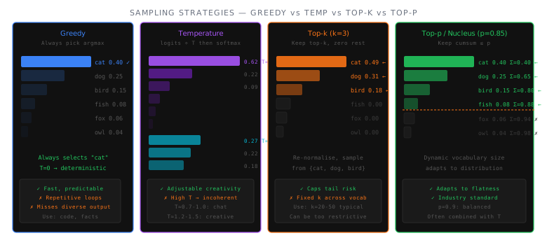
Four sampling strategy comparison: greedy always picks argmax; temperature scales logits; top-k keeps k most likely; top-p nucleus truncates by cumulative probability

Sampling strategies compared — from deterministic greedy to adaptive nucleus sampling

The simplest strategy: always pick the highest-probability token.

def greedy_decode(logits):
    """Always select the most likely token."""
    return torch.argmax(logits, dim=-1)  # [B]

Pros: Deterministic, fast. Cons: Repetitive, boring, can get stuck in loops. Never used for creative generation.

Temperature Scaling

Temperature controls the “sharpness” of the probability distribution. It scales the logits before softmax:

\[P(x_i) = \frac{\exp(z_i / \tau)}{\sum_j \exp(z_j / \tau)}\]

Temperature (τ)	Effect	Use Case
0.0	Greedy (argmax)	Not recommended (degenerate)
0.1–0.3	Very focused, near-deterministic	Code, math, factual QA
0.5–0.7	Balanced creativity + coherence	General chat, writing
0.8–1.0	More diverse, creative	Brainstorming, fiction
>1.0	Increasingly random	Rarely useful

def sample_with_temperature(logits, temperature=0.7):
    """Apply temperature scaling and sample."""
    if temperature == 0:
        return torch.argmax(logits, dim=-1)
    scaled = logits / temperature
    probs = torch.softmax(scaled, dim=-1)
    return torch.multinomial(probs, num_samples=1).squeeze(-1)

Top-k Sampling

Only consider the top k most probable tokens, zero out the rest:

def top_k_sampling(logits, k=50, temperature=1.0):
    """Keep only top-k tokens, zero out the rest."""
    scaled = logits / temperature
    top_k_values, _ = torch.topk(scaled, k, dim=-1)
    min_top_k = top_k_values[:, -1].unsqueeze(-1)
    scaled[scaled < min_top_k] = float('-inf')
    probs = torch.softmax(scaled, dim=-1)
    return torch.multinomial(probs, num_samples=1).squeeze(-1)

Problem: A fixed k doesn’t adapt to the model’s confidence. When the model is very confident (one token has 95% probability), k=50 still considers 50 tokens. When the model is uncertain, k=50 might miss important options.

Top-p (Nucleus) Sampling

Top-p (Holtzman et al., 2019) dynamically selects the smallest set of tokens whose cumulative probability exceeds p:

def top_p_sampling(logits, p=0.9, temperature=1.0):
    """Nucleus sampling — dynamic vocabulary size."""
    scaled = logits / temperature
    sorted_logits, sorted_indices = torch.sort(scaled, descending=True, dim=-1)
    cumulative_probs = torch.cumsum(torch.softmax(sorted_logits, dim=-1), dim=-1)

    # Remove tokens with cumulative prob above threshold
    sorted_mask = cumulative_probs - torch.softmax(sorted_logits, dim=-1) >= p
    sorted_logits[sorted_mask] = float('-inf')

    # Scatter back to original positions
    probs = torch.softmax(sorted_logits, dim=-1)
    indices = torch.multinomial(probs, num_samples=1)
    return sorted_indices.gather(-1, indices).squeeze(-1)

Top-p adapts: when confident, only 2–3 tokens might reach p=0.9. When uncertain, dozens of tokens contribute.

Beam Search

Beam search maintains B candidate sequences (“beams”) and expands the most promising ones:

beam_width = 3

Step 1: "The"   → [("The cat", 0.4), ("The dog", 0.3), ("The man", 0.2)]
Step 2: expand  → [("The cat sat", 0.35), ("The cat is", 0.33), ("The dog ran", 0.28)]
Step 3: expand  → ...select top 3 from all expansions...

Pros: Better for tasks with a single correct answer (translation). Cons: Tends to produce generic, high-probability text. Rarely used for open-ended generation.

Repetition Penalties

Without intervention, LLMs tend to repeat themselves. Several mechanisms help:

Penalty	Formula	Effect
Repetition penalty	`logits[token] /= penalty if token in seen`	Reduces probability of any previously generated token
Frequency penalty	`logits[token] -= freq_count * penalty`	Increases penalty the more a token appears
Presence penalty	`logits[token] -= penalty if token in seen`	Fixed penalty for any seen token (regardless of count)

Speculative Decoding

Speculative decoding uses a small “draft” model to propose multiple tokens, then the large model verifies them in a single forward pass:

Speculative Decoding

Draft model (1B): quickly generate K candidate tokens e.g., K=5 tokens in 5 fast passes

Target model (70B): verify all K tokens in one forward pass parallel evaluation

Accept matching tokens, reject from first mismatch keep 3–4 out of 5 on average

Net: 3–4 tokens per large-model forward pass instead of 1 ~2–3× speedup

The key property: speculative decoding produces exactly the same distribution as the target model — it’s a lossless speedup.

Structured Output / Constrained Decoding

Sometimes you need the model to output valid JSON, SQL, or match a schema. Constrained decoding masks the logits to only allow tokens that maintain validity:

# JSON mode: at each step, mask tokens that would produce invalid JSON
# If we're inside a string, only allow string-continuation tokens
# If we just saw a key, only allow ":"
# If we just saw a value, only allow "," or "}"

# Libraries: outlines, guidance, instructor
from outlines import models, generate

model = models.transformers("meta-llama/Llama-3.1-8B-Instruct")
generator = generate.json(model, schema)
result = generator("Extract the person's name and age from: ...")
# Guaranteed valid JSON matching the schema

Practical Configuration Guide

from transformers import GenerationConfig

# Factual / code (low creativity)
factual_config = GenerationConfig(
    max_new_tokens=512,
    temperature=0.1,
    top_p=0.9,
    do_sample=True,
    repetition_penalty=1.1,
)

# General chat (balanced)
chat_config = GenerationConfig(
    max_new_tokens=1024,
    temperature=0.7,
    top_p=0.9,
    top_k=50,
    do_sample=True,
    repetition_penalty=1.05,
)

# Creative writing (high diversity)
creative_config = GenerationConfig(
    max_new_tokens=2048,
    temperature=0.9,
    top_p=0.95,
    do_sample=True,
    repetition_penalty=1.15,
)

What’s Next

Every decode step reads the full KV-cache from memory. As sequences get longer, this becomes the dominant bottleneck. The next chapter dives deep into KV-cache mechanics — how it works, how much memory it uses, and why it matters.

← Previous: Chapter 15 — Alignment: RLHF & Beyond · Next: Chapter 17 — KV-Cache — Mechanics & Memory →

Last updated: April 2026